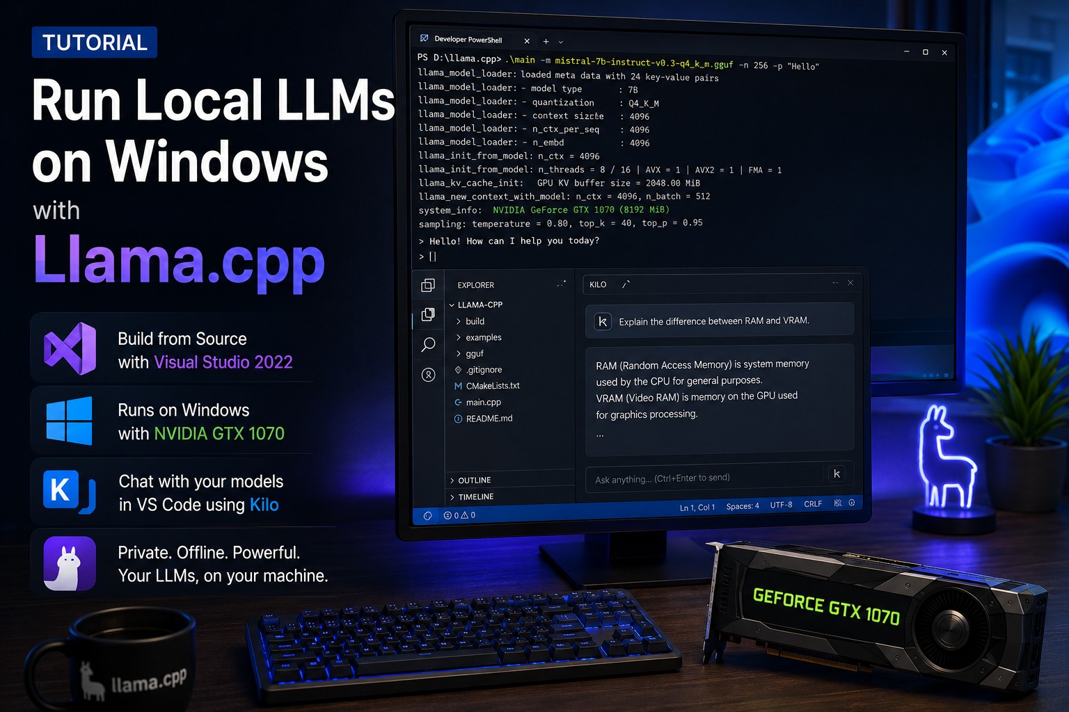
Compile and Run Local LLMs on Windows with llama.cpp, CUDA and Visual Studio 2022

Large Language Models (LLMs) no longer require expensive cloud subscriptions or high-end enterprise hardware. Thanks to projects like llama.cpp, it is possible to run modern quantized language models completely offline on a standard Windows PC.

In this article, we’ll build llama.cpp directly from the Git repository using Visual Studio 2022, enable CUDA support for an NVIDIA GeForce GTX 1070 (8 GB), and finally connect the local model to Kilo inside Visual Studio Code.

At the end of this tutorial you’ll have your own local AI coding assistant that never sends your source code to an external service.


]

Prerequisites

Before starting, make sure the following software is installed:

  • Windows 10 or Windows 11
  • Visual Studio 2022 with Desktop Development with C++
  • Git
  • CMake
  • NVIDIA CUDA 12.4 Toolkit
  • Visual Studio Code
  • Kilo VS Code extension

For this article the test system uses an NVIDIA GTX 1070 with 8 GB of VRAM. Although this GPU is several generations old, it is still perfectly capable of running modern 7B parameter models using 4-bit quantization.


Clone the llama.cpp Repository

Open PowerShell and clone the official repository.

git clone https://github.com/ggml-org/llama.cpp.git
cd llama.cpp

Using the latest Git repository instead of precompiled binaries ensures that you always have the newest features, performance improvements and bug fixes.


Compile llama.cpp with CUDA Support

Since we want to use our NVIDIA GPU, CUDA support must be enabled during compilation.

The GTX 1070 is based on the Pascal architecture which has Compute Capability 6.1, therefore we explicitly specify the CUDA architecture during configuration.

Generate the build files:

cmake -B build -DGGML_CUDA=ON -DCMAKE_CUDA_ARCHITECTURES="61"

Now compile the project.

cmake --build build --config Release

Depending on your computer this process usually takes several minutes.

After a successful build you’ll find all executables inside

cd build\bin\Release

including

  • llama-cli.exe
  • llama-server.exe
  • llama-bench.exe
  • llama-quantize.exe

Download a Model

For this tutorial we’ll use the excellent Qwen2.5-Coder-7B-Instruct model in GGUF format from huggingface.

Download Link (qwen2.5-coder-7b-instruct-q4_k_m.gguf)

Store the model in

C:\sw\models

Using a dedicated model directory makes it easy to switch between different models later.


Start the Local LLM Server

Start the server with the following command:

cd C:\src\llama.cpp\build\bin\Release\
.\llama-server.exe `
    -m "C:\sw\models\qwen2.5-coder-7b-instruct-q4_k_m.gguf" `
    -c 16384 `
    -ngl 99

Let’s briefly explain these parameters.

ParameterDescription
-mPath to the GGUF model
-c 16384Context window of 16K tokens
-ngl 99Offload as many transformer layers as possible to the GPU

When the server starts successfully you should see log messages indicating that CUDA has been initialized and that the model has been loaded.

The server exposes an OpenAI-compatible REST API on port 8080, making it compatible with many AI tools.


Install Kilo Code

Open Visual Studio Code and install the Kilo Code extension from the Marketplace.

Kilo Code is an AI coding assistant capable of communicating with OpenAI-compatible APIs. Instead of connecting to a cloud provider, we’ll point it to our own llama.cpp server running locally.


Configure Kilo Code

Configure the OpenAI-compatible provider so that Kilo connects to your local server instead of an online service. Go to Settings => Providers => Custom provider => Connect

  • Provider ID: llamacpp
  • Display Name: llamacpp
  • Provider API: OpenAI Compatible
  • Base URL: http://localhost:8080
  • API Key: dummy
  • Name of the model: qwen2.5-coder


The API key is ignored by llama.cpp but many clients expect one to be configured.

Open the Kilo configuration file (Global Config / kilo.jsonc) and modify your local model.

{
  "models": {
    "C:\\sw\\models\\qwen2.5-coder-7b-instruct-q4_k_m.gguf": {
      "name": "qwen2.5-coder",
      "limit": {
        "context": 16384,
        "output": 4096
      }
    }
  }
}

Once the configuration has been saved, restart Visual Studio Code if necessary.


Test the Installation

Open Kilo Code and start a new conversation (Make sure the correct model is selected).

As a first test, ask the model:

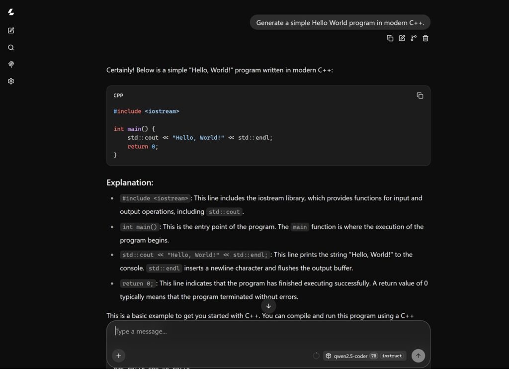
Generate a simple Hello World program in modern C++.

The generated response should look similar to this:

#include 

int main()
{
    std::cout << "Hello World!" << std::endl;
    return 0;
}

If Kilo Code produces a valid C++ program, your complete local AI environment is working correctly.


Alternative Interfaces

If there are problems with the Client (Kilo Code) there are several other options to test or use the LLM

Using the Llama.cpp web interface

With this URL you can also use the local LLM: http://127.0.0.1:8080
Using Cline as a client

Install cline as a VS Code extension, then open the Cline settings and select OpenAI Compatible as the provider.

Configure the endpoint as follows:

SettingValue
Base URLhttp://127.0.0.1:8080
API Keydummy
ModelC:\sw\models\qwen2.5-coder-7b-instruct-q4_k_m.gguf

The API key is not validated by llama-server, but Cline requires a value to be entered.

Once the configuration has been saved, Cline immediately connects to the local server.

Using Claude CLI as a client

First create a claude config file for the current user:

# run in PowerShell
$null = mkdir "$env:USERPROFILE\.claude" -Force
@'
{
  "env": {
    "ANTHROPIC_BASE_URL": "http://127.0.0.1:8080",
    "ANTHROPIC_AUTH_TOKEN": "sk-dummy-value",
    "CLAUDE_CODE_AUTO_COMPACT_WINDOW": "14000",
    "CLAUDE_AUTOCOMPACT_PCT_OVERRIDE": "70",
    "CLAUDE_CODE_DISABLE_1M_CONTEXT": "1"
  },
  "disableBundledSkills": true,
  "disableWorkflows": true,
  "permissions": {
    "deny": [
      "Workflow", "NotebookEdit", "CronCreate", "CronDelete",
      "CronList", "AskUserQuestion", "EnterPlanMode", "ExitPlanMode"
    ]
  }
}
'@ | Out-File "$env:USERPROFILE\.claude\settings.json" -Encoding utf8

Now we can start claude by running claude in the PowerShell Window:

claude

Performance Notes

The NVIDIA GTX 1070 may not be the newest graphics card, but it still performs remarkably well with quantized 7B models.

The Q4_K_M quantization offers an excellent compromise between model quality, memory consumption and inference speed.

If you encounter CUDA out-of-memory errors, consider lowering the context size or using fewer GPU layers. Conversely, systems with newer GPUs and more VRAM can increase these values for improved performance.


Getting the latest llama.cpp version

To get the latest version of llama.cpp from the git repository perform the following steps in a PowerShell window:

cd C:\src\llama.cpp\
git pull
Remove-Item -Path .\build -Recurse -Force

Now recompile llama.cpp as described here.


References

Why Use Local LLMs?

Running your own language model offers several important advantages.

  • Complete privacy
  • No monthly API costs
  • Offline operation
  • Low latency
  • Full control over model selection
  • No rate limits

For developers working with proprietary source code or confidential customer projects, local inference can be an attractive alternative to cloud-based AI services.


Conclusion

Compiling llama.cpp from source gives you the latest optimizations and full control over the build process. Combined with CUDA acceleration, even an older graphics card such as the GTX 1070 can provide an enjoyable experience with modern coding models like Qwen2.5-Coder-7B-Instruct.

Once the local server is connected to Kilo Code, Visual Studio Code gains a private AI coding assistant that works entirely on your own machine. Whether you’re generating boilerplate code, explaining existing projects or experimenting with new ideas, this setup delivers a fast and secure development environment without relying on external AI providers.

Happy coding!
0
PostGIS Leaflet

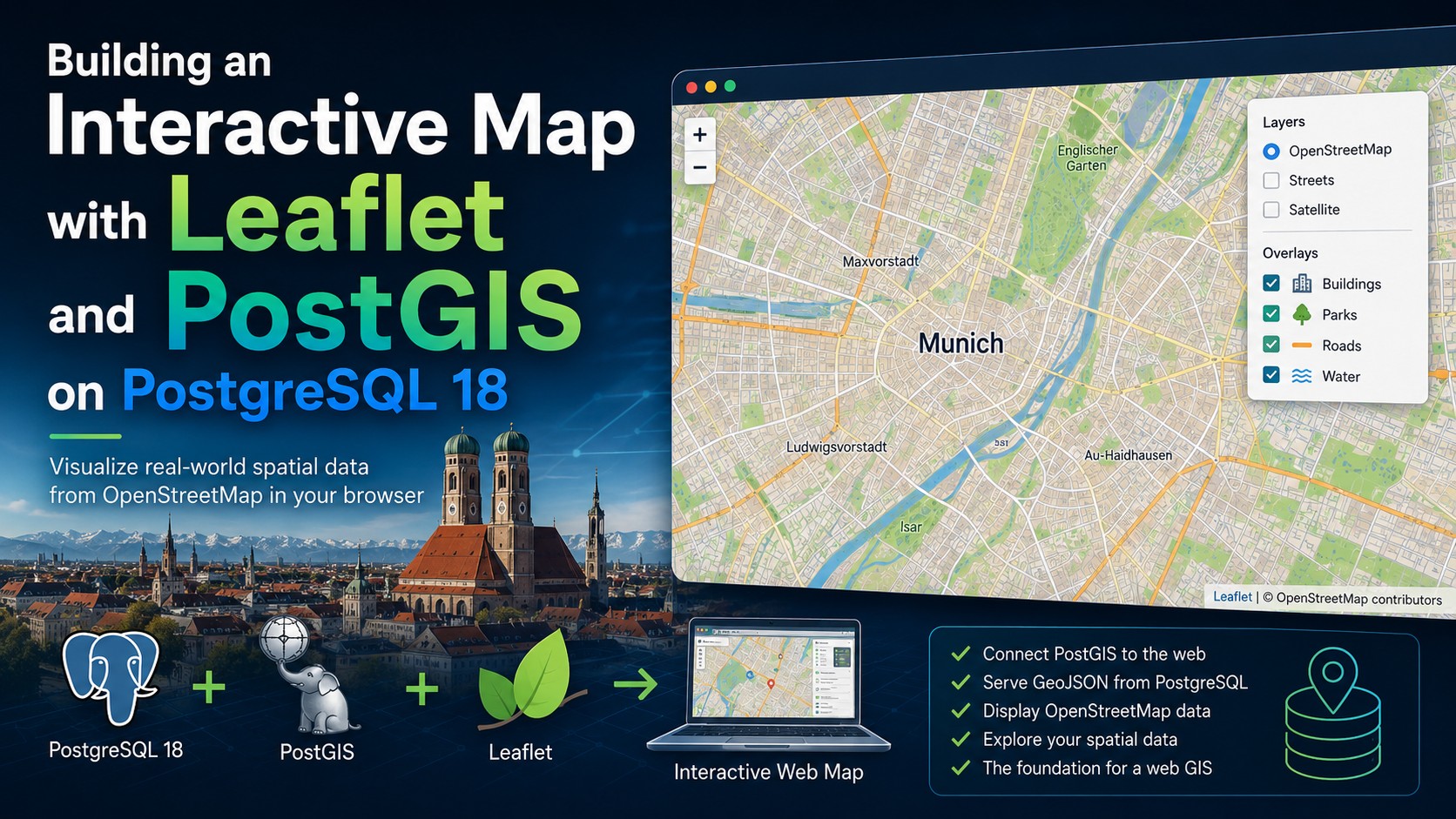
Building an Interactive Map with Leaflet and PostGIS on PostgreSQL 18

In the previous article, Building a Production-Ready PostGIS Environment on PostgreSQL 18, we installed PostGIS, created a spatial database, and imported OpenStreetMap data. While querying the database with SQL is useful, spatial data becomes much more valuable once it can be visualized on an interactive map.

In this article, we’ll build a simple web application using Leaflet, the most popular open-source JavaScript mapping library. The application will retrieve data directly from PostgreSQL/PostGIS and display it on an interactive OpenStreetMap layer. This environment will become the foundation for future articles covering performance tuning, GiST indexes, query optimization, monitoring, and database maintenance.


Architecture

Our application consists of four components:

Browser
    │
    ▼
Leaflet (JavaScript)
    │
    ▼
PHP Web Server
    │
    ▼
PostgreSQL 18 + PostGIS

The browser requests GeoJSON data from a PHP script, which executes a SQL query against PostgreSQL and returns the results in JSON format.


Prerequisites

This article assumes you already have:

  • PostgreSQL 18 installed
  • PostGIS enabled
  • OpenStreetMap data imported using osm2pgsql

If not, please read the previous article first.


Installing Apache and PHP

On RHEL 10 install Apache, PHP and the PostgreSQL driver and perform additional tasks.

# install packages
dnf -y install httpd php php-pgsql
# enable Apache
systemctl enable httpd --now
# open the firewall
firewall-cmd --add-service=http --permanent
firewall-cmd --reload

Preparing PostgreSQL

Create a dedicated database user for the web application.

# run as the postgres user
psql gisdemo <<EOF
-- create role
CREATE ROLE leaflet LOGIN PASSWORD 'changeme';
-- grant access
GRANT CONNECT ON DATABASE gisdemo TO leaflet;
GRANT USAGE ON SCHEMA public TO leaflet;
GRANT SELECT ON ALL TABLES IN SCHEMA public TO leaflet;
\q
EOF


Creating the GeoJSON API

Create the following file as root

mkdir /var/www/html/api
vi /var/www/html/api/parks.php

with the following content:

<?php

$conn = pg_connect("
host=localhost
dbname=gisdemo
user=leaflet
password=changeme
");

$sql = "
SELECT
  json_build_object(
    'type','FeatureCollection',
    'features', json_agg(feature)
  )
FROM (
  SELECT
    json_build_object(
      'type','Feature',
      'geometry', ST_AsGeoJSON(ST_Transform(way, 4326))::json,
      'properties', json_build_object('name',name,'type',leisure)
    ) feature
  FROM planet_osm_polygon
  WHERE leisure='park'
    AND ST_DWithin(
          ST_Transform(way, 4326)::geography,
          ST_SetSRID(ST_MakePoint(11.576124, 48.137154), 4326)::geography,
          10000   -- 10 km radius
        )
) t;
";

$result = pg_query($conn, $sql);
header("Content-Type: application/json");
echo pg_fetch_result($result, 0, 0);
?>

To test the endpoint point a browser to:

http://lin6.fritz.box/api/parks.php

You should receive a GeoJSON FeatureCollection.


Creating the Leaflet Application

Create the following file as the root user

vi /var/www/html/index.html

with this content:

<!DOCTYPE html>
<html>
<head>
<meta charset="utf-8">
<title>Leaflet + PostGIS</title>
<link rel="stylesheet" href="https://unpkg.com/leaflet/dist/leaflet.css" />
<style>
html, body { height:100%; margin:0; }
#map { height:100%; }
</style>
</head>
<body>
<div id="map"></div>
<script src="https://unpkg.com/leaflet/dist/leaflet.js"></script>
<script>
const map = L.map('map').setView([48.137154, 11.576124], 12);

L.tileLayer('https://tile.openstreetmap.org/{z}/{x}/{y}.png', {
    maxZoom: 19,
    attribution: '© OpenStreetMap contributors'
}).addTo(map);

fetch('api/parks.php')
    .then(response => response.json())
    .then(data => {
        console.log('Received GeoJSON:', data); // Check console
        const layer = L.geoJSON(data, {
            style: { color: 'green', weight: 2, fillOpacity: 0.5 },
            onEachFeature: function(feature, layer) {
                layer.bindPopup(feature.properties.name || 'Unnamed park');
            }
        }).addTo(map);

        // Zoom to the data extent
        const bounds = layer.getBounds();
        if (bounds.isValid()) {
            map.fitBounds(bounds);
            console.log('Zoomed to data bounds');
        } else {
            console.warn('No valid bounds from data');
        }
    })
    .catch(err => console.error('Fetch error:', err));
</script>
</body>
</html>

Viewing the Map

Point your browser to:

http://lin6.fritz.box/

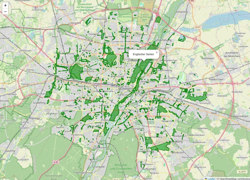
You should now see:

  • OpenStreetMap
  • Munich
  • Parks imported from OpenStreetMap
  • Clickable polygons
  • Popups displaying park names

Unlike many tutorials, every object displayed comes directly from your OpenStreetMap import.


Understanding the Data Flow

The request follows a simple path.

Browser

↓

Leaflet

↓

parks.php

↓

PostgreSQL

↓

PostGIS

↓

ST_AsGeoJSON()

↓

GeoJSON

↓

Leaflet

The browser never communicates directly with PostgreSQL. Instead, PHP acts as a lightweight API that retrieves spatial data and converts it into GeoJSON.


Why GeoJSON?

GeoJSON has become the standard format for exchanging geographic information between databases and web applications.

Advantages include:

  • Native Leaflet support
  • Human-readable JSON
  • Generated directly by PostGIS
  • Supported by most GIS software
  • Lightweight and easy to debug

Exploring the Database

Let’s execute a few SQL statements to understand the imported dataset.

How many parks are available?

psql gisdemo <<EOF
SELECT count(*)
FROM planet_osm_polygon
WHERE leisure='park';
EOF
Sample Output (click to expand):
[postgres@lin6 ~]$ psql gisdemo <<EOF
SELECT count(*)
FROM planet_osm_polygon
WHERE leisure='park';
EOF
 count
-------
  6247
(1 row)

[postgres@lin6 ~]$

List some park names.

psql gisdemo <<EOF
SELECT
    name
FROM planet_osm_polygon
WHERE leisure='park'
ORDER BY name
LIMIT 20;
EOF
Sample Output (click to expand):
[postgres@lin6 ~]$ psql gisdemo <<EOF
SELECT
    name
FROM planet_osm_polygon
WHERE leisure='park'
ORDER BY name
LIMIT 20;
EOF
                          name
--------------------------------------------------------
 1A Hundegarten Kompetenzzentrum und Hundenasenparadies
 Abdurrahim-Özüdoğru-Park
 Aberdeenpark
 Abloner-Garten
 Achenpark
 Achenseeplatz
 Achenseeplatz
 Adamiwiese
 Adelheidpark
 AGFA-Park
 Ägidienplatz
 Ägidiuspark
 Agricolaplatz
 Aktiv Park
 Aktiv-Park
 Albert-Schweitzer-Park
 Albert-Schweitzer-Seniorenzentrum
 Albin-Lang-Stadtpark Landshut
 Alfons Halbig Platz
 Alfred-Dick-Park
(20 rows)

[postgres@lin6 ~]$

Calculate the area of the English Garden.

psql gisdemo <<EOF
SELECT 
  name,
  round(ST_Area(ST_Transform(way, 4326)::geography)) AS square_meters
FROM planet_osm_polygon
WHERE name = 'Englischer Garten'
ORDER BY square_meters DESC
LIMIT 1;
EOF
Output (click to expand):
[postgres@lin6 ~]$ psql gisdemo <<EOF
SELECT
  name,
  round(ST_Area(ST_Transform(way, 4326)::geography)) AS square_meters
FROM planet_osm_polygon
WHERE name = 'Englischer Garten'
ORDER BY square_meters DESC
LIMIT 1;
EOF
       name        | square_meters
-------------------+---------------
 Englischer Garten |       3931062
(1 row)

[postgres@lin6 ~]$

These examples demonstrate that PostGIS is much more than a storage engine—it provides advanced spatial analysis directly within PostgreSQL.


Preparing for Performance Tuning

The application is intentionally simple, but it already gives us a realistic workload that we can optimize.

In the upcoming articles we’ll use this same application to demonstrate:

  • GiST indexes
  • Bounding box queries
  • ST_DWithin
  • ST_Intersects
  • EXPLAIN ANALYZE
  • VACUUM
  • REINDEX
  • Autovacuum tuning
  • Streaming Replication
  • Backup and recovery
  • Monitoring

Every optimization will be measured by observing how quickly the map loads.


What’s Next?

In the next article we’ll investigate why some spatial queries become slow as the amount of OpenStreetMap data increases.

We’ll create our first GiST index, compare execution plans with EXPLAIN ANALYZE, and measure the impact on map loading times.


Conclusion

By combining PostgreSQL, PostGIS, OpenStreetMap, and Leaflet, we’ve built the foundation of a real-world GIS application. Rather than relying on artificial sample data, our application visualizes actual OpenStreetMap features stored in PostgreSQL, making it an ideal environment for exploring spatial queries, database administration, and performance tuning.

This architecture closely resembles those used by municipalities, utility companies, logistics providers, and many enterprise GIS platforms. Throughout the remainder of this series, we’ll continue extending and optimizing this application while learning how PostgreSQL and PostGIS handle large-scale spatial workloads.

0
Debugging PostgreSQL with VS Code

Debugging PostgreSQL with Visual Studio Code

Debugging a database system often requires looking beyond SQL statements and configuration parameters. When investigating complex issues, understanding what happens inside the PostgreSQL source code can provide valuable insights into query execution, process behavior and internal database mechanisms. For developers, contributors and advanced database administrators, the ability to step through PostgreSQL code can significantly simplify troubleshooting and performance analysis.

Read More

0
SQL Server Patching

Patching SQL Server

Keeping Microsoft SQL Server environments secure and up to date is one of the most important responsibilities of every SQL Server DBA and infrastructure team. Regular security patching not only helps protect critical business data against newly discovered vulnerabilities, but also improves system stability, reliability and compliance with modern security standards.

In this blog post, we will look at best practices for securing and patching SQL Server environments.

Read More

0