Measuring PostgreSQL per process I/O throughput
PostgreSQL provides excellent monitoring capabilities, but sometimes you need to know something more specific:
Which PostgreSQL process is responsible for the current disk I/O?
With two small Checkmk scripts, you can monitor the I/O throughput of individual PostgreSQL processes and visualize the results directly in Checkmk.
Why monitor PostgreSQL process I/O?
Looking only at the overall database I/O can make it difficult to understand what is happening on a busy PostgreSQL server. Different PostgreSQL processes have very different responsibilities. For example:
client_backendprocesses handle client connectionscheckpointerwrites dirty buffers to diskbgwriterperforms background writeswalwriterwrites WAL datawalsenderprocesses handle WAL streamingautovacuum_workerprocesses perform automatic maintenanceparallel workersand PostgreSQLI/O workerscan also contribute significantly to the I/O load
Having these processes visible separately in Checkmk makes unusual I/O activity much easier to identify.
The Checkmk local check
The first script is:
/usr/lib/check_mk_agent/local/check_pg_process_io.sh
The script reads the Linux process I/O counters from:
/proc/<pid>/io
For each PostgreSQL process, it determines the process role, for example checkpointer, walwriter, autovacuum_worker or client_backend.
Processes belonging to the same role are aggregated. The script stores the previous cumulative counters and calculates the difference over time to determine the current I/O throughput in bytes per second.
Both read and write throughput are exported as Checkmk performance data.
Script: (click to expand)
#!/usr/bin/bash
# ---------------------------------------------------------------------------
# Checkmk local check: per-process disk I/O for all PostgreSQL processes.
#
# Emits ONE service whose perfdata contains both read and write metrics:
#   read_bytes_<role>   -> graph "PostgreSQL process read I/O"
#   write_bytes_<role>  -> graph "PostgreSQL process write I/O"
# One line per PostgreSQL role in each graph.
#
# IMPORTANT: perfdata items are separated by '|' (pipe), as required by the
# Checkmk local check protocol.
#
# Install: /usr/lib/check_mk_agent/local/check_pg_process_io.sh  (chmod 0700)
# Requires: bash 4+, Checkmk agent running as root (to read /proc/<pid>/io)
# ---------------------------------------------------------------------------

# ---------------------------- CONFIG ---------------------------------------
PG_USER="postgres"
WARN_BPS=$((10 * 1024 * 1024))     # 10 MB/s per series
CRIT_BPS=$((50 * 1024 * 1024))     # 50 MB/s per series
SKIP_NON_SERVER_PROCS="true"       # true  -> drop psql / bash / (sd-pam)
STATE_ROOT="/var/lib/check_mk_agent/pg_proc_io"
SERVICE_NAME="PostgreSQL process I/O"
# ---------------------------------------------------------------------------

NOW=$(date +%s)
mkdir -p "$STATE_ROOT/read_bytes" "$STATE_ROOT/write_bytes" 2>/dev/null

# Map a cmdline like "postgres: 18/main: checkpointer process" to a stable
# role label such as "checkpointer". Handles PG 9.x .. 18+ naming schemes,
# PG 18 io workers / walsummarizer, and PG 18 client backends (which no
# longer use the "client backend" keyword on the cmdline).
#
# Returns non-zero if the process should be skipped.
normalize_role() {
    local cmd
    cmd=$(printf '%s' "$1" \
        | sed -E 's/^postgres:[[:space:]]*//' \
        | sed -E 's/^[0-9]+(\/[^:[:space:]]+)?:[[:space:]]*//' \
        | sed -E 's/[[:space:]]+process$//' \
        | sed -E 's/[[:space:]]+$//')

    case "$cmd" in
        # --- named PostgreSQL roles -------------------------------------
        "background writer")                     echo "bgwriter";;
        "autovacuum worker"*)                    echo "autovacuum_worker";;
        "autovacuum launcher")                   echo "autovacuum_launcher";;
        "logical replication launcher")          echo "logical_replication_launcher";;
        "logical replication tablesync worker"*) echo "logical_replication_tablesync_worker";;
        "logical replication worker"*)           echo "logical_replication_worker";;
        "parallel worker"*)                      echo "parallel_worker";;
        "checkpointer")                          echo "checkpointer";;
        "walwriter")                             echo "walwriter";;
        "walsender")                             echo "walsender";;
        "walreceiver")                           echo "walreceiver";;
        "archiver")                              echo "archiver";;
        "startup")                               echo "startup";;

        # --- PostgreSQL 18+ new process types ---------------------------
        "io worker "*)                           echo "$(printf '%s' "$cmd" | tr ' ' '_')";;
        "walsummarizer")                         echo "walsummarizer";;

        # --- postmaster (raw binary path, no "postgres:" prefix) -------
        */bin/postgres\ -*)                      echo "postmaster";;
        "postgres"|"")                           echo "postmaster";;

        # --- non-server processes owned by the postgres user -----------
        "psql"*|"bash"|"sh"|"-bash"|"-sh"|"(sd-pam)"|"sd-pam")
            if [ "$SKIP_NON_SERVER_PROCS" = "true" ]; then
                return 1
            fi
            printf '%s' "$cmd" | sed 's/[^A-Za-z0-9_]/_/g'
            ;;

        # --- anything else with multiple fields = client backend --------
        *[[:space:]]*)                           echo "client_backend";;

        # --- truly unknown: sanitised as-is ----------------------------
        *) printf '%s' "$cmd" | sed 's/[^A-Za-z0-9_]/_/g';;
    esac
}

# -------- Collect cumulative read/write counters per role --------
declare -A READ_TOTALS=()
declare -A WRITE_TOTALS=()

for PID in $(pgrep -u "$PG_USER" 2>/dev/null); do
    IO_FILE="/proc/$PID/io"
    [ -r "$IO_FILE" ] || continue

    R=$(awk '/^read_bytes:/  {print $2}' "$IO_FILE" 2>/dev/null)
    W=$(awk '/^write_bytes:/ {print $2}' "$IO_FILE" 2>/dev/null)
    [ -z "$R" ] && continue
    [ -z "$W" ] && W=0

    CMD=$(tr '\0' ' ' < "/proc/$PID/cmdline" 2>/dev/null | sed 's/[[:space:]]*$//')
    [ -z "$CMD" ] && CMD=$(cat "/proc/$PID/comm" 2>/dev/null)

    ROLE=$(normalize_role "$CMD") || continue

    # All PIDs of the same role are summed into one metric.
    READ_TOTALS[$ROLE]=$(( ${READ_TOTALS[$ROLE]:-0} + R ))
    WRITE_TOTALS[$ROLE]=$(( ${WRITE_TOTALS[$ROLE]:-0} + W ))
done

if [ "${#READ_TOTALS[@]}" -eq 0 ]; then
    echo "3 \"$SERVICE_NAME\" - No readable PostgreSQL processes (agent must run as root)"
    exit 0
fi

# -------- Compute rates and build perfdata --------
# Perfdata items are separated by '|' (pipe), as required by Checkmk.
PERFDATA=""
WORST=0

compute_rate() {
    local STATE_FILE="$1" CUR="$2"
    local LAST=0 LAST_TS=0
    if [ -f "$STATE_FILE" ]; then
        read -r LAST LAST_TS < "$STATE_FILE" 2>/dev/null || true
        LAST=${LAST:-0}; LAST_TS=${LAST_TS:-0}
    fi
    printf '%s %s\n' "$CUR" "$NOW" > "$STATE_FILE"
    [ "$LAST_TS" -eq 0 ] && return
    local DT=$((NOW - LAST_TS))
    [ "$DT" -le 0 ] && return
    local DB=$((CUR - LAST))
    [ "$DB" -lt 0 ] && DB=0
    echo $((DB / DT))
}

for ROLE in "${!READ_TOTALS[@]}"; do
    R_RATE=$(compute_rate "$STATE_ROOT/read_bytes/$ROLE"  "${READ_TOTALS[$ROLE]}")
    W_RATE=$(compute_rate "$STATE_ROOT/write_bytes/$ROLE" "${WRITE_TOTALS[$ROLE]:-0}")

    [ -n "$R_RATE" ] && PERFDATA="${PERFDATA}read_bytes_${ROLE}=${R_RATE}B/s;${WARN_BPS};${CRIT_BPS}|"
    [ -n "$W_RATE" ] && PERFDATA="${PERFDATA}write_bytes_${ROLE}=${W_RATE}B/s;${WARN_BPS};${CRIT_BPS}|"

    for RATE in "$R_RATE" "$W_RATE"; do
        [ -z "$RATE" ] && continue
        if   [ "$RATE" -ge "$CRIT_BPS" ]; then WORST=2
        elif [ "$RATE" -ge "$WARN_BPS" ] && [ "$WORST" -lt 2 ]; then WORST=1
        fi
    done
done

# -------- Drop state for roles that no longer exist --------
for METRIC_DIR in "$STATE_ROOT/read_bytes" "$STATE_ROOT/write_bytes"; do
    for f in "$METRIC_DIR"/*; do
        [ -f "$f" ] || continue
        base=$(basename "$f")
        keep=0
        for ROLE in "${!READ_TOTALS[@]}"; do
            [ "$ROLE" = "$base" ] && keep=1 && break
        done
        [ "$keep" -eq 0 ] && rm -f "$f"
    done
done

case $WORST in
    2) TXT="CRITICAL";;
    1) TXT="WARNING";;
    *) TXT="OK";;
esac

if [ -z "$PERFDATA" ]; then
    echo "0 \"$SERVICE_NAME\" - Initializing (waiting for second sample)"
    exit 0
fi

# Strip the trailing pipe
PERFDATA="${PERFDATA%|}"

echo "$WORST \"$SERVICE_NAME\" ${PERFDATA} ${TXT} - read/write bytes/s per PostgreSQL process"
Configurable thresholds
The script uses configurable warning and critical thresholds:
WARN_MBPS=10
CRIT_MBPS=50
This allows Checkmk to report a warning or critical state when an individual PostgreSQL process role exceeds the configured I/O throughput.
The Checkmk agent must run with sufficient privileges to read /proc/<pid>/io.
The Checkmk graphing plugin
The second script is:
~/local/lib/python3/cmk_addons/plugins/pg_process_io/graphing/pg_process_io.py (owner: mon group: mon file mode: 0600)
This Python plugin defines the Checkmk metrics for the different PostgreSQL process roles and creates two graphs.
Script: (click to expand):
#!/usr/bin/env python3
# ~/local/lib/python3/cmk_addons/plugins/pg_process_io/graphing/pg_process_io.py
# s.a. https://docs.checkmk.com/plugin-api/latest/cmk.graphing/v1.graphs.html#cmk.graphing.v1.graphs.Graph

from cmk.graphing.v1 import Title
from cmk.graphing.v1.graphs import Graph, MinimalRange
from cmk.graphing.v1.metrics import Color, IECNotation, Metric, Unit

UNIT_BPS = Unit(IECNotation("B/s"))

# ---------------------------------------------------------------
# Read metrics (one per PostgreSQL role)
# ---------------------------------------------------------------
metric_read_bytes_postmaster = Metric(
    name="read_bytes_postmaster",
    title=Title("Read postmaster"),
    unit=UNIT_BPS,
    color=Color.LIGHT_RED,
)
metric_read_bytes_checkpointer = Metric(
    name="read_bytes_checkpointer",
    title=Title("Read checkpointer"),
    unit=UNIT_BPS,
    color=Color.RED,
)
metric_read_bytes_bgwriter = Metric(
    name="read_bytes_bgwriter",
    title=Title("Read bgwriter"),
    unit=UNIT_BPS,
    color=Color.DARK_RED,
)
metric_read_bytes_walwriter = Metric(
    name="read_bytes_walwriter",
    title=Title("Read walwriter"),
    unit=UNIT_BPS,
    color=Color.LIGHT_ORANGE,
)
metric_read_bytes_walsender = Metric(
    name="read_bytes_walsender",
    title=Title("Read walsender"),
    unit=UNIT_BPS,
    color=Color.ORANGE,
)
metric_read_bytes_walreceiver = Metric(
    name="read_bytes_walreceiver",
    title=Title("Read walreceiver"),
    unit=UNIT_BPS,
    color=Color.DARK_ORANGE,
)
metric_read_bytes_archiver = Metric(
    name="read_bytes_archiver",
    title=Title("Read archiver"),
    unit=UNIT_BPS,
    color=Color.LIGHT_YELLOW,
)
metric_read_bytes_startup = Metric(
    name="read_bytes_startup",
    title=Title("Read startup"),
    unit=UNIT_BPS,
    color=Color.YELLOW,
)
metric_read_bytes_io_worker_0 = Metric(
    name="read_bytes_io_worker_0",
    title=Title("Read io_worker_0"),
    unit=UNIT_BPS,
    color=Color.DARK_YELLOW,
)
metric_read_bytes_io_worker_1 = Metric(
    name="read_bytes_io_worker_1",
    title=Title("Read io_worker_1"),
    unit=UNIT_BPS,
    color=Color.LIGHT_GREEN,
)
metric_read_bytes_io_worker_2 = Metric(
    name="read_bytes_io_worker_2",
    title=Title("Read io_worker_2"),
    unit=UNIT_BPS,
    color=Color.GREEN,
)
metric_read_bytes_walsummarizer = Metric(
    name="read_bytes_walsummarizer",
    title=Title("Read walsummarizer"),
    unit=UNIT_BPS,
    color=Color.DARK_GREEN,
)
metric_read_bytes_autovacuum_launcher = Metric(
    name="read_bytes_autovacuum_launcher",
    title=Title("Read autovacuum_launcher"),
    unit=UNIT_BPS,
    color=Color.LIGHT_BLUE,
)
metric_read_bytes_autovacuum_worker = Metric(
    name="read_bytes_autovacuum_worker",
    title=Title("Read autovacuum_worker"),
    unit=UNIT_BPS,
    color=Color.BLUE,
)
metric_read_bytes_logical_replication_launcher = Metric(
    name="read_bytes_logical_replication_launcher",
    title=Title("Read logical_replication_launcher"),
    unit=UNIT_BPS,
    color=Color.DARK_BLUE,
)
metric_read_bytes_logical_replication_worker = Metric(
    name="read_bytes_logical_replication_worker",
    title=Title("Read logical_replication_worker"),
    unit=UNIT_BPS,
    color=Color.LIGHT_CYAN,
)
metric_read_bytes_logical_replication_tablesync_worker = Metric(
    name="read_bytes_logical_replication_tablesync_worker",
    title=Title("Read logical_replication_tablesync_worker"),
    unit=UNIT_BPS,
    color=Color.CYAN,
)
metric_read_bytes_parallel_worker = Metric(
    name="read_bytes_parallel_worker",
    title=Title("Read parallel_worker"),
    unit=UNIT_BPS,
    color=Color.DARK_CYAN,
)
metric_read_bytes_client_backend = Metric(
    name="read_bytes_client_backend",
    title=Title("Read client_backend"),
    unit=UNIT_BPS,
    color=Color.LIGHT_PURPLE,
)

# ---------------------------------------------------------------
# Write metrics (one per PostgreSQL role)
# ---------------------------------------------------------------
metric_write_bytes_postmaster = Metric(
    name="write_bytes_postmaster",
    title=Title("Write postmaster"),
    unit=UNIT_BPS,
    color=Color.LIGHT_RED,
)
metric_write_bytes_checkpointer = Metric(
    name="write_bytes_checkpointer",
    title=Title("Write checkpointer"),
    unit=UNIT_BPS,
    color=Color.RED,
)
metric_write_bytes_bgwriter = Metric(
    name="write_bytes_bgwriter",
    title=Title("Write bgwriter"),
    unit=UNIT_BPS,
    color=Color.DARK_RED,
)
metric_write_bytes_walwriter = Metric(
    name="write_bytes_walwriter",
    title=Title("Write walwriter"),
    unit=UNIT_BPS,
    color=Color.LIGHT_ORANGE,
)
metric_write_bytes_walsender = Metric(
    name="write_bytes_walsender",
    title=Title("Write walsender"),
    unit=UNIT_BPS,
    color=Color.ORANGE,
)
metric_write_bytes_walreceiver = Metric(
    name="write_bytes_walreceiver",
    title=Title("Write walreceiver"),
    unit=UNIT_BPS,
    color=Color.DARK_ORANGE,
)
metric_write_bytes_archiver = Metric(
    name="write_bytes_archiver",
    title=Title("Write archiver"),
    unit=UNIT_BPS,
    color=Color.LIGHT_YELLOW,
)
metric_write_bytes_startup = Metric(
    name="write_bytes_startup",
    title=Title("Write startup"),
    unit=UNIT_BPS,
    color=Color.YELLOW,
)
metric_write_bytes_io_worker_0 = Metric(
    name="write_bytes_io_worker_0",
    title=Title("Write io_worker_0"),
    unit=UNIT_BPS,
    color=Color.DARK_YELLOW,
)
metric_write_bytes_io_worker_1 = Metric(
    name="write_bytes_io_worker_1",
    title=Title("Write io_worker_1"),
    unit=UNIT_BPS,
    color=Color.LIGHT_GREEN,
)
metric_write_bytes_io_worker_2 = Metric(
    name="write_bytes_io_worker_2",
    title=Title("Write io_worker_2"),
    unit=UNIT_BPS,
    color=Color.GREEN,
)
metric_write_bytes_walsummarizer = Metric(
    name="write_bytes_walsummarizer",
    title=Title("Write walsummarizer"),
    unit=UNIT_BPS,
    color=Color.DARK_GREEN,
)
metric_write_bytes_autovacuum_launcher = Metric(
    name="write_bytes_autovacuum_launcher",
    title=Title("Write autovacuum_launcher"),
    unit=UNIT_BPS,
    color=Color.LIGHT_BLUE,
)
metric_write_bytes_autovacuum_worker = Metric(
    name="write_bytes_autovacuum_worker",
    title=Title("Write autovacuum_worker"),
    unit=UNIT_BPS,
    color=Color.BLUE,
)
metric_write_bytes_logical_replication_launcher = Metric(
    name="write_bytes_logical_replication_launcher",
    title=Title("Write logical_replication_launcher"),
    unit=UNIT_BPS,
    color=Color.DARK_BLUE,
)
metric_write_bytes_logical_replication_worker = Metric(
    name="write_bytes_logical_replication_worker",
    title=Title("Write logical_replication_worker"),
    unit=UNIT_BPS,
    color=Color.LIGHT_CYAN,
)
metric_write_bytes_logical_replication_tablesync_worker = Metric(
    name="write_bytes_logical_replication_tablesync_worker",
    title=Title("Write logical_replication_tablesync_worker"),
    unit=UNIT_BPS,
    color=Color.CYAN,
)
metric_write_bytes_parallel_worker = Metric(
    name="write_bytes_parallel_worker",
    title=Title("Write parallel_worker"),
    unit=UNIT_BPS,
    color=Color.DARK_CYAN,
)
metric_write_bytes_client_backend = Metric(
    name="write_bytes_client_backend",
    title=Title("Write client_backend"),
    unit=UNIT_BPS,
    color=Color.LIGHT_PURPLE,
)

# ---------------------------------------------------------------
# Combined graphs
# ---------------------------------------------------------------
graph_pg_process_read_bytes = Graph(
    name="pg_process_read_bytes",
    title=Title("PostgreSQL process read I/O"),
    simple_lines=[
        "read_bytes_archiver",
        "read_bytes_autovacuum_launcher",
        "read_bytes_autovacuum_worker",
        "read_bytes_bgwriter",
        "read_bytes_checkpointer",
        "read_bytes_client_backend",
        "read_bytes_io_worker_0",
        "read_bytes_io_worker_1",
        "read_bytes_io_worker_2",
        "read_bytes_logical_replication_launcher",
        "read_bytes_logical_replication_tablesync_worker",
        "read_bytes_logical_replication_worker",
        "read_bytes_parallel_worker",
        "read_bytes_postmaster",
        "read_bytes_startup",
        "read_bytes_walreceiver",
        "read_bytes_walsender",
        "read_bytes_walsummarizer",
        "read_bytes_walwriter",
    ],
    optional=[
        "read_bytes_archiver",
        "read_bytes_autovacuum_launcher",
        "read_bytes_autovacuum_worker",
        "read_bytes_bgwriter",
        "read_bytes_checkpointer",
        "read_bytes_client_backend",
        "read_bytes_io_worker_0",
        "read_bytes_io_worker_1",
        "read_bytes_io_worker_2",
        "read_bytes_logical_replication_launcher",
        "read_bytes_logical_replication_tablesync_worker",
        "read_bytes_logical_replication_worker",
        "read_bytes_parallel_worker",
        "read_bytes_postmaster",
        "read_bytes_startup",
        "read_bytes_walreceiver",
        "read_bytes_walsender",
        "read_bytes_walsummarizer",
        "read_bytes_walwriter",
    ],
)

graph_pg_process_write_bytes = Graph(
    name="pg_process_write_bytes",
    title=Title("PostgreSQL process write I/O"),
    simple_lines=[
        "write_bytes_archiver",
        "write_bytes_autovacuum_launcher",
        "write_bytes_autovacuum_worker",
        "write_bytes_bgwriter",
        "write_bytes_checkpointer",
        "write_bytes_client_backend",
        "write_bytes_io_worker_0",
        "write_bytes_io_worker_1",
        "write_bytes_io_worker_2",
        "write_bytes_logical_replication_launcher",
        "write_bytes_logical_replication_tablesync_worker",
        "write_bytes_logical_replication_worker",
        "write_bytes_parallel_worker",
        "write_bytes_postmaster",
        "write_bytes_startup",
        "write_bytes_walreceiver",
        "write_bytes_walsender",
        "write_bytes_walsummarizer",
        "write_bytes_walwriter",
    ],
    optional=[
        "write_bytes_archiver",
        "write_bytes_autovacuum_launcher",
        "write_bytes_autovacuum_worker",
        "write_bytes_bgwriter",
        "write_bytes_checkpointer",
        "write_bytes_client_backend",
        "write_bytes_io_worker_0",
        "write_bytes_io_worker_1",
        "write_bytes_io_worker_2",
        "write_bytes_logical_replication_launcher",
        "write_bytes_logical_replication_tablesync_worker",
        "write_bytes_logical_replication_worker",
        "write_bytes_parallel_worker",
        "write_bytes_postmaster",
        "write_bytes_startup",
        "write_bytes_walreceiver",
        "write_bytes_walsender",
        "write_bytes_walsummarizer",
        "write_bytes_walwriter",
    ],
)
PostgreSQL process read I/O
The first graph shows the read throughput of the individual PostgreSQL process types.
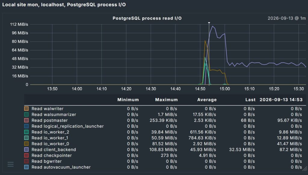
This makes it possible to see, for example, whether a sudden increase in database read activity is coming from client backends, autovacuum workers, the checkpointer or another PostgreSQL process.
PostgreSQL process write I/O
The second graph shows the corresponding write throughput.
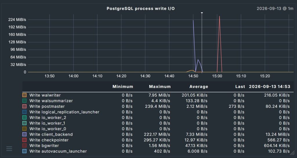
This is particularly useful when investigating high write activity caused by checkpoints, WAL processing, autovacuum or application workloads.
What you get in Checkmk
The local check creates a Checkmk service called: PostgreSQL process I/O
The service provides performance data for the different PostgreSQL process roles. The graphing plugin then presents the data as two separate graphs:
PostgreSQL process read I/O
and
PostgreSQL process write I/O
Instead of looking at a single aggregated database I/O value, you can see which PostgreSQL process role is responsible for the activity.
Supported PostgreSQL processes
The graphing plugin includes metrics for process types such as:
postmastercheckpointerbgwriterwalwriterwalsenderwalreceiverarchiverstartupio_worker_0io_worker_1io_worker_2walsummarizerautovacuum_launcherautovacuum_workerlogical_replication_launcherlogical_replication_workertablesync_workerparallel_workerclient_backend
This also makes the solution useful across PostgreSQL versions where additional background processes are present.
Conclusion
Monitoring PostgreSQL I/O per process provides another useful level of visibility for database performance analysis. With check_pg_process_io.sh and pg_process_io.py, Checkmk can show read and write throughput for individual PostgreSQL process roles. This makes troubleshooting high I/O activity much easier and helps answer a practical question:
Which PostgreSQL process is currently causing high I/O load?
For PostgreSQL administrators using Checkmk, this is a relatively small addition that can provide valuable insight when investigating database performance and storage activity.